SP2 - Understanding Objects

The introductory tutorial stopped short of going into the customary way SoundProcesses is used, and instead showed the transactional variant of ScalaCollider to play a synth. Most of the time, instead of creating instances of Synth yourself, you will instead manipulate other objects that automatically spawn synths when the server is running and some other conditions are met. In this second tutorial I will introduce this approach to creating sounding objects.

The Core Object: Proc

The SoundProcesses way of referring to a synth is an object of type Proc. The function of Proc is threefold:

• its method graph points to the SynthGraph, and it is variable that can be updated
• its method outputs points to an interface for creating outlets that can be patched into other objects (not used in this tutorial)
• it implements the Obj trait or “protocol”, a uniform way all sorts of objects are modelled in SoundProcesses

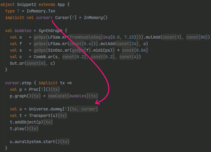
Before I explain what this means, let us look at another example snippet Snippet2 that shows the usage of Proc:

copyimport de.sciss.lucre.Cursor
import de.sciss.lucre.synth.InMemory
import de.sciss.proc.{Proc, Transport, Universe}
import de.sciss.synth._
import de.sciss.synth.Import._
import de.sciss.synth.ugen._

object Snippet2 extends App {
  type T = InMemory.Txn
  implicit val cursor: Cursor[T] = InMemory()

  val bubbles = SynthGraph {
    val o   = LFSaw.kr(Seq(8.0, 7.23)).mulAdd(3, 80)
    val f   = LFSaw.kr(0.4).mulAdd(24, o)
    val s   = SinOsc.ar(f.midiCps) * 0.04
    val c   = CombN.ar(s, 0.2, 0.2, 4)
    Out.ar(0, c)
  }

  cursor.step { implicit tx =>
    val p = Proc[T]()
    p.graph() = bubbles

    val u = Universe.dummy[T]
    val t = Transport(u)
    t.addObject(p)
    t.play()

    u.auralSystem.start()
  }

  Thread.sleep(10000)
  sys.exit()
}

If you run this snippet, you should see SuperCollider booting, then hear the familiar ‘analog bubbles’ sound again. Also a significant portion of the code is identical to the first version we’ve seen in the previous tutorial. The main difference here is that instead of waiting for the aural system to have booted and then create a Synth instance, an instance of Proc is created and added to a Transport. I will discuss the changes step by step, beginning with the initialisation:

copytype T = InMemory.Txn
implicit val cursor: Cursor[T] = InMemory()

The first line contains a so-called type-alias. In Scala, a type-alias does not create a new type, but simply introduces a new name for an existing type. In SoundProcesses, many objects require as type parameter the type of transaction—in-memory, durable, confluent—and we can avoid having to insert the particular transaction type we choose, here InMemory.Txn, in many places. So in the following lines, whenever you see the application of [T], this is just aliased to [InMemory.Txn]. However, should we eventually decide to change the transaction type, for example to Durable.Txn, the only change that needs to be made to the program is to rewrite the type-alias as type T = Durable.Txn. Don’t confuse T as a type parameter in the definition of a method and class, with T as an alias to a concrete type used in the invocation of a method or instantiation of class. We just happen to use the same letter T which is short and easy to remember.

The next line adds an implicit modifier to the cursor, and we also annotate the value type explicitly with Cursor[T]. The reason for marking this value implicit is that when the Universe object is created further down, it requires an implicit parameter of type Cursor[T], and we therefore make it visible here, so the compiler will find it. In IntelliJ, you can enable View > Show Implicit Hints to see when Scala actually uses implicit parameters:

The type annotation : Cursor[T] is not necessary, strictly speaking, because Scala will otherwise infer the type automatically. But it is good practice to always specify the types of implicit values, because it avoids surprises and ambiguities in the compiler’s search for implicit values. We could also have chosen to use the more precise type : InMemory here, but we never need to refer to this value as this particular system, so the more general type is sufficient and therefore better indicates the use case.

Instantiating and Configuring Proc

Next, let’s see the creation of the Proc instance:

copyval p = Proc[T]()
p.graph() = bubbles

It may not be obvious that Proc[S]() instantiates a class, so let’s look at the signature of what’s being called here:

object Proc {
  def apply[T <: Txn[T]]()(implicit tx: T): Proc[T] ...
}

This is the companion object of the trait (type) Proc. Often we create instances of classes and traits not through new ClassName but through a method on their companion object. This is the case here. But should that call then not have been Proc.apply[T]()?

We had used this before with other types: Creating the in-memory system via InMemory() is nothing but InMemory.apply(), a call of the apply method in InMemory’s companion object. The same with SynthGraph {} (we can drop the parentheses here, because the argument is a function, although parameterless).

Next is p.graph() = bubbles. The graph method is defined as follows:

def graph: Proc.GraphObj.Var[T]

There is another, related shortcut here in Scala. The call we’re making is actually p.graph.update(bubbles), where update is a method on the Proc.GraphObj.Var type, which I will talk about in a second. So when a method on some object x is def update(v: A): Unit, we can use the alternative syntax x() = v. This is really cool, because we can define mutable cells or variables that way:

copytrait Cell[A] {  // fictitious type
  def apply(): A
  def update(v: A): Unit
}

With such definition, we could write:

copyval cell: Cell[Int] = ???   // imagine we had such cell
val oldValue = cell()       // aka cell.apply()
val newValue = oldValue + 1
cell() = newValue           // aka cell.update(newValue)

Scala uses this principle in many cases. Take for example arrays:

copyval xs = Array(3, 5, 8, 0)
xs(3) = xs(1) + xs(2)  // aka xs.update(3, xs.apply(1) + xs.apply(2))
assert(xs(3) == 13)

This also works when we have an additional implicit argument list. This is the case for SynthGraphObj.Var which is an extension of Var:

copytrait Var[Tx, A] {
  def apply()(implicit tx: Tx): A
  def update(v: A)(implicit tx: Tx): Unit
}

What is the element type A in the case of Proc.GraphObj.Var? It is Proc.GraphObj. It is defined as follows:

trait GraphObj[T <: Txn[T]] extends Expr[T, SynthGraph]

The type Expr[T, A] is ubiquitous in SoundProcesses.

There are many types of expressions in SoundProcesses, for example IntObj[T] which is an Expr[T, Int], StringObj[T] which is an Expr[T, String], BooleanObj[T] which is an Expr[T, Boolean], and so on. Expressions usually include a constant sub-type that simply wraps the primitive value, a variable type that holds another expression of the same type that can be exchanged, and often also unary and binary operations—for example, in the case of IntObj, the unary negation or the binary addition of two integer expressions. Expressions are reactive in that they participate in SoundProcesses’ event dispatch system. If the value of an expression changes, that information propagates along all objects that observe the expression. So when we write p.graph() = bubbles—i.e. we call the update method of the expression variable graph of type GraphObj.Var—the new value stored in that expression will be detected by any other object in the system watching that expression variable. If the process was playing on the sound synthesis server, the layer that is responsible for the playback would be notified that the graph changed and thus replace the old synth with a new synth.

There is only one last bit to explain in the synth-graph assignment: An expression variable must be updated with an expression of the same type, so GraphObj here. But it seems as if we can put a primitive value of type SynthGraph here directly, namely bubbles. In order to avoid ceremony, SoundProcesses permits this by automatically lifting primitive values to their respective expressions. So the call performed really is

p.graph.update(Proc.GraphObj.newConst[T](bubbles))

Obviously, writing p.graph() = bubbles is much nicer. The next snippet will make this mechanism perhaps more obvious, as we update numeric expressions controlling a synthesis parameter.

Attribute Map of an Obj

Both Expr and Proc are sub-types of Obj, the basic unit of (possibly stateful) objects in SoundProcesses. Obj defines the following properties:

• an id method that gives a unique value, the format of which depends on the transaction type T chosen. This identifier is used for example in the database persistence, when the system is durable.
• it can be persisted, i.e. written to and read from a workspace database
• a dispose method allows us to remove an object from our system, freeing observers and resources associated with it.
• the changed method gives access to an event bus system for monitoring changes to the object
• most relevant to us, the attr method gives access to a dictionary associated with the object, the so-called attribute map with type AttrMap.

Using the attribute map, it is easy to annotate objects with additional information. It’s SoundProcesses’ way of contextualising objects and linking them together. The concept of a heterogeneous dictionary is well known from dynamically typed languages. It is a simple way to extend the otherwise determined interface (methods) of an object. On the downside, attribute maps work by means of convention: The keys into this dictionary are ordinary strings, so we lose a bit of type safety by using the dictionary, as we must ensure ourselves that we use the correct keys for retrieving a particular type of information. If we mistyped the attribute’s key or name, the map would not return the value we were looking for.

Before explaining this concept in more detail, we shall first look at an example Snippet3 of using the attribute map of a Proc. The most common case is to store control values here for use within the synth-graph function:

copyimport de.sciss.lucre.synth.InMemory
import de.sciss.lucre.{Cursor, DoubleObj}
import de.sciss.proc.{Proc, Transport, Universe}
import de.sciss.synth._
import de.sciss.synth.Import._
import de.sciss.synth.ugen._

object Snippet3 extends App {
  type T = InMemory.Txn
  implicit val cursor: Cursor[T] = InMemory()

  val bubbles = SynthGraph {
    import de.sciss.synth.proc.graph.Ops._
    val f0  = "freq".kr
    val o   = LFSaw.kr(Seq(f0, f0 * 8/7.23)).mulAdd(3, 80)
    val f   = LFSaw.kr(0.4).mulAdd(24, o)
    val s   = SinOsc.ar(f.midiCps) * 0.04
    val c   = CombN.ar(s, 0.2, 0.2, 4)
    Out.ar(0, c)
  }

  val pH = cursor.step { implicit tx =>
    val p = Proc[T]()
    p.graph() = bubbles
    p.attr.put("freq", DoubleObj.newConst(8.0))

    val u = Universe.dummy[T]
    val t = Transport(u)
    t.addObject(p)
    t.play()

    u.auralSystem.start()
    tx.newHandle(p)
  }

  Thread.sleep(8000)

  cursor.step { implicit tx =>
    val p = pH()
    p.attr.put("freq", DoubleObj.newConst(0.1))
  }

  Thread.sleep(6000)

  sys.exit()
}

If you run this, you will hear the familiar analog bubbles, but after a few seconds, the frequency modulation frequency changes from 8.0 to a very low value of 0.1. The following changes have been applied in the transition from Snippet2 to Snippet3. Inside the synth-graph definition:

copyimport de.sciss.synth.proc.graph.Ops._
val f0  = "freq".kr

The syntax "freq".kr might be familiar from ScalaCollider. There, it was enabled by importing de.sciss.synth.Ops.stringToControl, creating control proxies for setting and updating synth parameters from the client. In SoundProcesses, we use a different import that enables the same syntax, but different implementation. Here, the layer that creates the synth from the Proc looks up control values in the Proc’s attribute map. Different types of values are supported, the most basic one being an IntObj or DoubleObj for numeric scalar values. Here we set the initial value that will be picked up by the synth:

copyp.attr.put("freq", DoubleObj.newConst(8.0))

The attribute key "freq" is purely by convention, we could have used a different name, but we must ensure that we refer to the same key inside the synth-graph function, otherwise the value would not be found. Here, the automatic lifting from the primitive 8.0 to a DoubleObj does not kick in, because the Scala compiler has no idea what kind of Obj we want to create. That is the reason why we have to explicitly construct that object through DoubleObj.newConst. The type parameter T is inferred however, as it is required by a Proc[T], so we do not have to repeat it.

We use a “poor man’s procedure” to update the attribute eight seconds (8000 milliseconds) later. We must be careful not to block the transaction, so Thread.sleep is placed between two separate calls to cursor.step. We can overwrite the previous attribute value by simply using another p.attr.put with the same key. One thing looks very odd, and that’s this at the periphery:

copyval pH = cursor.step { implicit tx =>
  val p = Proc[T]()
  // ...
  tx.newHandle(p)
}

// ...

cursor.step { implicit tx =>
  val p = pH()
  p.attr.put("freq", DoubleObj.newConst(0.1))
}

Note how the original assignment val p = Proc[T]() is inside the first cursor.step block, so that local variable would not be visible in the next cursor.step block. We therefore return something from the first block to the outer scope, so we can use it again in the next nested scope. Why did we not just write:

copyval p = cursor.step { implicit tx =>
  val p0 = Proc[T]()
  // ...
  p0 // this is the functions return value and thus becomes the outer `p`
}

// ...

cursor.step { implicit tx =>
  p.attr.put("freq", DoubleObj.newConst(0.1))
}

? To be clear, this would indeed have worked in this case! There is however one system, Confluent, where we have to “refresh” transactional objects if we use them across different transactions. The mechanism by which that is done is to return from the transaction where an object was created a special handle obtained through tx.newHandle(obj). Then, in successive transactions, we can get a refreshed version of that object by calling apply() on that handle.

Universe and Transport

The last change in Snippet3 is to create and start a transport:

copyval u = Universe.dummy[T]
val t = Transport(u)
t.addObject(p)
t.play()

The Transport type is a way to connect object “models” to their “aural views”, in other words, to turn data into actual sound. Unlike a Synth, which you can only create when there is a booted server, a Proc can be created at any point. It is simply a description of a sound. In order to hear that sound, it must be turned into what SoundProcesses calls an aural view. The transport class takes care of this translation. A side effect of this design is that you can have multiple sounding representations of the same model at the same time.

A transport is created with a “universe” as parameter. A Universe is a context that holds together various useful things, such as a handle to workspace, a scheduler, an aural-system, etc. We do not use an actual workspace here, so we can shortcut its creation by using Universe.dummy. Normally, a Workspace allows objects to register callbacks for when the workspace closes. For example, the transport registers itself with a workspace in order to ensure that it stops and frees resources if the corresponding workspace closes.

After the transport has been instantiated, you add objects for which you wish to have aural representations created. Finally, you use the transport’s methods play() and stop() to tell it you want to start and stop listening to these objects. You can call play even before the server is booted, and the transport will internally start scheduling objects, but they only become sound when the server is ready as well. That happens in our example, it thus takes less than the eight seconds between first hearing the bubbles and their frequency changing, because there is a delay from u.auralSystem.start() to the server actually having booted. It we did not want that, we’d have to defer the t.play() call and the Thread.sleep until the moment that the aural system was booted.

Using a Scheduler

As a final exercise of this tutorial, another more lengthy Snippet4 will shows us how to replace the “poor man’s” approach with a “proper” way of scheduling temporal events. To begin with, here is the full code:

copyimport de.sciss.lucre.synth.InMemory
import de.sciss.lucre.{Cursor, DoubleObj, Source}
import de.sciss.proc.{Proc, Scheduler, TimeRef, Transport, Universe}
import de.sciss.synth._
import de.sciss.synth.Import._
import de.sciss.synth.ugen._

object Snippet4 extends App {
  type T = InMemory.Txn
  implicit val cursor: Cursor[T] = InMemory()

  val bubbles = SynthGraph {
    import de.sciss.synth.proc.graph.Ops._
    val p0  = "pitch".kr(80.0)
    val o   = LFSaw.kr(Seq(1.0, 7.23/8)).mulAdd(3, p0)
    val f   = LFSaw.kr(0.4).mulAdd(4, o)
    val s   = SinOsc.ar(f.midiCps) * 0.04
    val c   = CombN.ar(s, 0.2, 0.2, 2)
    Out.ar(0, c)
  }

  class PitchMod(sch: Scheduler[T], pchH: Source[T, DoubleObj.Var[T]]) {
    def iterate()(implicit tx: T): Unit = {
      val pch = pchH()
      pch() = math.random() * 40 + 60
      sch.schedule(sch.time + TimeRef.SampleRate.toLong) { implicit tx =>
        iterate()
      }
    }
  }

  cursor.step { implicit tx =>
    val p = Proc()
    p.graph() = bubbles
    val pch = DoubleObj.newVar(0.0)
    p.attr.put("pitch", pch)

    val u   = Universe.dummy[T]
    val t   = Transport(u)
    val sch = t.scheduler
    val mod = new PitchMod(sch, tx.newHandle(pch))
    mod.iterate()
    t.addObject(p)
    t.play()

    u.auralSystem.start()
  }
}

If you run this, you will hear a variant of the bubbles with the pitch changing every second. The program will run indefinitely, until you press the stop button in IntelliJ. The first change compared to Snippet3 is to the synth-graph itself. Instead of modulating the modulator frequency, we now use a control p0 for the fundamental pitch itself:

copyval p0  = "pitch".kr(80.0)
val o   = LFSaw.kr(Seq(1.0, 7.23/8)).mulAdd(3, p0)

Also, the other modulations are toned down to be able to better hear those changes. The pitch is a midi note value, which formerly had been a constant of 80. Here is how we store the value in the attribute map, this time using an expression variable that we can update instead of overwriting the attribute map entry again:

copyval pch = DoubleObj.newVar(0.0)
p.attr.put("pitch", pch)

Remember that DoubleObj.newVar(0.0) is shorthand for DoubleObj.newVar[T](DoubleObj.newConst[T](0.0)) (in some cases, the transaction type parameter T is also automatically inferred by Scala). The initial value of 0.0 does not matter, as we’re going to change it few lines further down: We are creating an instance of an auxiliary class PitchMod with its parameters being the scheduler of the transport, available through t.scheduler and a transactional handle of the double expression variable just created. This class, that we created ourselves in the code, has a method iterate which is called once:

copyval sch = t.scheduler
val mod = new PitchMod(sch, tx.newHandle(pch))
mod.iterate()

Because that class will reschedule itself and create new transactions, we’re on the safe side by using tx.newHandle(pch), although as said before, this is not strictly necessary if the system is in-memory. Now let’s see what our class is doing:

copyclass PitchMod(sch: Scheduler[T], pchH: Source[T, DoubleObj.Var[T]]) {
  def iterate()(implicit tx: T): Unit = {
    val pch = pchH()
    pch() = math.random() * 40 + 60
    sch.schedule(sch.time + TimeRef.SampleRate.toLong) { implicit tx =>
      iterate()
    }
  }
}

First, you can see what the type of the transactional handle is: Source[T, DoubleObj.Var[T]]. An Source (the handle) has a single method apply() that returns a fresh version of the encapsulated object. The transactional iterate method does exactly that in its first line, it creates a fresh version of the pitch variable val pch = pchH(), then updates it with a random value. math is an object that belongs to the Scala standard library and lives in the scala. package, so we can use it directly without import. The random() method emits a pseudo-random Double number between 0.0 (inclusive) and 1.0 (exclusive), very much what 1.0.rand would do in SuperCollider. With the multiplication and addition, we bring it into the range of 60 to 100; as a midi pitch, that means we produce a frequency between 261.6 Hz and 2637.0 Hz. The system that maintains the synth for the proc sees this update and automatically adjusts the control value inside the UGen graph.

The schedule method of the Scheduler is straight forward:

def schedule(time: Long)(fun: T => Unit)(implicit tx: T): Int

The first argument list consists of one argument for the time of the scheduled event, in the second list, there is an argument for a function that takes a new transaction. The function’s return type is Unit, that means the scheduler does not do anything with the return value of the function, the function is merely executed for its side-effects (although, since we use transactions, it’s not really fair to speak of “side” effects). Remember that, as we use a lambda or function literal, we can drop the parentheses and write sch.schedule(x) { implicit tx => ... } instead of sch.schedule(x)({ implicit tx => ... }).

The third argument list takes an implicit transaction, which means that schedule can only be called from within an ongoing transaction. The scheduler is designed with a logical clock that is guaranteed to remain constant throughout a transaction. That logical clock can be queried using the time method. Since schedule’s own time argument designates an absolute point in time, in order to schedule something with a given delay, we can simply add the current time to the desired delay.

schedule returns an Int token we could use to cancel the scheduled function if we wanted to.

TimeRef.SampleRate is given as a Double, but we can write .toLong to get the long integer representation. It should be clear now that sch.time + TimeRef.SampleRate.toLong means that we schedule an event exactly one second into the future. If we wanted to schedule it 1.5 seconds into the future, we could have written sch.time + (1.5 * TimeRef.SampleRate).toLong. The function executed when the scheduled event arrives, is simply calling iterate again, therefore repeating the process of setting a random pitch and scheduling the next period.

It may have been surprising that we can define a custom class PitchMod anywhere in the source code. This is part of Scala’s philosophy of regularity—it allows you to introduce any of its abstractions within the context where you need them, and it does not introduce artificial restrictions on where those abstractions can be defined. PitchMod really is just a helper created for this particular case here, grouping together data—the scheduler instance and the expression variable—with behaviour—the iterate method.